Breaking down barriers to scale: How we've optimized Elasticsearch usage at Intercom

Elasticsearch is an indispensable part of Intercom.

It underpins core Intercom features like Inbox, Inbox Views, API, Articles, the user list, reporting, Resolution Bot, and our internal logging systems. Our Elasticsearch clusters contain more than 350TB of customer data, store more than 300 billion documents, and serve more than 60 thousand requests per second at peak.

As Intercom’s Elasticsearch usage increases, we need to ensure our systems scale to support our continued growth. With the recent launch of our next-generation Inbox, Elasticsearch’s reliability is more critical than ever.

We decided to tackle a problem with our Elasticsearch setup that posed an availability risk and threatened future downtime: uneven distribution of traffic/work between the nodes in our Elasticsearch clusters.

Early signs of inefficiency: Load imbalance

Elasticsearch allows you to scale horizontally by increasing the number of nodes that store data (data nodes). We began to notice a load imbalance among these data nodes: some of them were under more pressure (or “hotter”) than others due to higher disk or CPU usage.

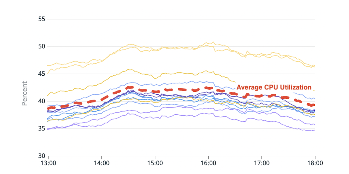
(Fig. 1) Imbalance in CPU usage: Two hot nodes with ~20% higher CPU utilization than the average.

Elasticsearch’s built-in shards placement logic makes decisions based on a calculation that roughly estimates the available disk space in each node and number of shards of an index per node. Resource utilization by shard does not factor into this calculation. As a result, some nodes could receive more resource-hungry shards and become “hot”. Every search request is processed by multiple data nodes, so a hot node that is pushed over its limits during peak traffic can cause performance degradation for the whole cluster.

A common reason for hot nodes is the shard placement logic assigning large shards (based on disk utilization) to clusters, making a balanced allocation less likely. Typically, a node might be assigned one large shard more than the others, making it hotter in disk utilization. The presence of large shards also hinders our ability to incrementally scale the cluster, as adding a data node doesn’t guarantee load reduction from all hot nodes (Fig. 2).

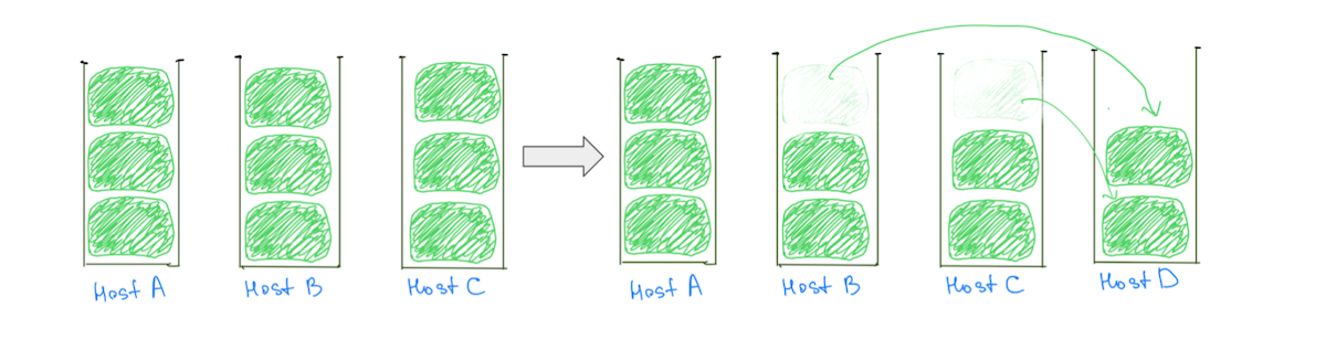
(Fig. 2) Adding a data node hasn’t resulted in load reduction on Host A. Adding another node would reduce the load on Host A, but the cluster will still have uneven load distribution.

In contrast, having smaller shards helps reduce the load on all data nodes as the cluster scales – including the “hot” ones (Fig. 3).

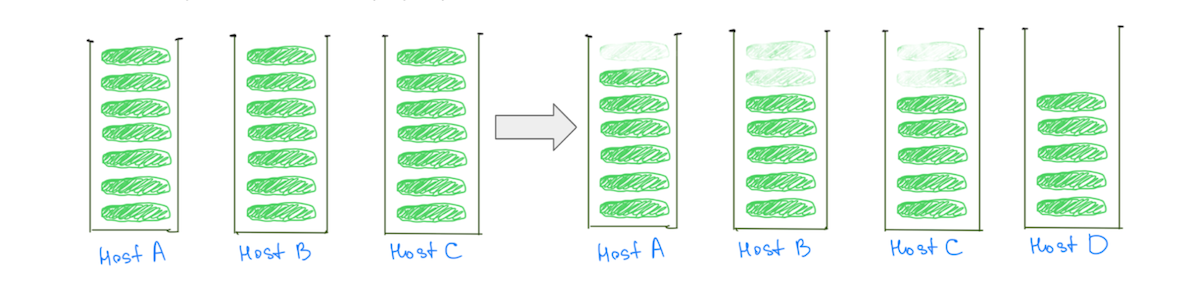
(Fig. 3) Having many smaller shards helps reduce the load on all data nodes.

Note: the problem isn’t limited to clusters with large-sized shards. We would observe a similar behavior if we replace “size” with “CPU utilization” or “search traffic”, but comparing sizes makes it easier to visualize.

As well as impacting cluster stability, load imbalance affects our ability to scale cost-effectively. We will always have to add more capacity than needed to keep the hotter nodes below dangerous levels. Fixing this problem would mean better availability and significant cost savings from utilizing our infrastructure more efficiently.

Our deep understanding of the problem helped us realize that the load could be distributed more evenly if we had:

• More shards relative to the number of data nodes. This would ensure that most nodes received an equal number of shards.
• Smaller shards relative to the size of the data nodes, so that even if some nodes were given a few extra shards, it wouldn’t result in any meaningful increase in load for those nodes.

Cupcake solution: Fewer bigger nodes

This ratio of the number of shards to the number of data nodes, and the size of the shards to the size of the data nodes, can be tweaked by having a larger number of smaller shards. But it can be tweaked more easily by moving to fewer but bigger data nodes.

We decided to start with a cupcake to verify this hypothesis. We migrated a few of our clusters to bigger, more powerful instances with fewer nodes – preserving the same total capacity. For example, we moved a cluster from 40 4xlarge instances to 10 16xlarge instances, reducing the load imbalance by distributing the shards more evenly.

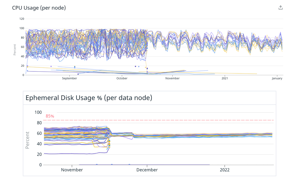
(Fig. 4) Better load distribution across disk and CPU by moving to fewer bigger nodes.

The fewer bigger nodes mitigation validated our assumptions that tweaking the number and size of the data nodes can improve load distribution. We could have stopped there, but there were some downsides to the approach:

• We knew the load imbalance would crop up again as shards grow larger over time, or if more nodes were added to the cluster to account for increased traffic.
• Bigger nodes make incremental scaling more expensive. Adding a single node would now cost more, even if we only needed a little extra capacity.

Challenge: Crossing the Compressed Ordinary Object Pointers (OOPs) threshold

Moving to fewer bigger nodes was not as simple as just changing the instance size. A bottleneck we faced was preserving the total heap size available (heap size on one node x total number of nodes) as we migrated.

We had been capping the heap size in our data nodes to ~30.5 GB, as suggested by Elastic, to make sure we stayed below the cutoff so the JVM could use compressed OOPs. If we capped the heap size to ~30.5 GB after moving to fewer, bigger nodes, we would reduce our heap capacity overall as we would be working with fewer nodes.

“The instances we were migrating to were huge and we wanted to assign a large portion of the RAM to the heap so that we had space for the pointers, with enough left for the filesystem cache”

We couldn’t find a lot of advice about the impact of crossing this threshold. The instances we were migrating to were huge and we wanted to assign a large portion of the RAM to the heap so that we had space for the pointers, with enough left for the filesystem cache. We experimented with a few thresholds by replicating our production traffic to test clusters, and settled on ~33% to ~42% of the RAM as the heap size for machines with more than 200 GB of RAM.

The change in heap size impacted various clusters differently. While some clusters showed no change in metrics like “JVM % heap in use” or “Young GC Collection Time”, the general trend was an increase. Regardless, overall it was a positive experience, and our clusters have been running for more than 9 months with this configuration – without any issues.

Long-term fix: Many smaller shards

A longer-term solution would be to move towards having a larger number of smaller shards relative to the number and size of data nodes. We can get to smaller shards in two ways:

• Migrating the index to have more primary shards: this distributes the data in the index among more shards.
• Breaking down the index into smaller indexes (partitions): this distributes the data in the index among more indexes.

It’s important to note we don’t want to create a million tiny shards, or have hundreds of partitions. Every index and shard requires some memory and CPU resources.

“We focused on making it easier to experiment and fix suboptimal configurations within our system, rather than fixating on the ‘perfect’ configuration”

In most cases, a small set of large shards uses fewer resources than many small shards. But there are other options – experimentation should help you reach a more suitable configuration for your use case.

To make our systems more resilient, we focused on making it easier to experiment and fix suboptimal configurations within our system, rather than fixating on the “perfect” configuration.

Partitioning indexes

Increasing the number of primary shards can sometimes impact performance for queries that aggregate data, which we experienced while migrating the cluster responsible for Intercom’s Reporting product. In contrast, partitioning an index into multiple indexes distributes the load onto more shards without degrading query performance.

Intercom has no requirement for co-locating data for multiple customers, so we chose to partition based on customers’ unique IDs. We also decided to partition based on the modulus of the customers’ IDs, which helped us deliver value faster by simplifying the partitioning logic and reducing required setup.

“To partition the data in a way that least impacted our engineers’ existing habits and methods, we first invested a lot of time into understanding how our engineers use Elasticsearch”

To partition the data in a way that least impacted our engineers’ existing habits and methods, we first invested a lot of time into understanding how our engineers use Elasticsearch. We deeply integrated our observability system into the Elasticsearch client library and swept our codebase to learn about all the different ways our team interacts with Elasticsearch APIs.

Our failure-recovery mode was to retry requests, so we made required changes where we were making non-idempotent requests. We ended up adding some linters to discourage usage of APIs like `update/delete_by_query`, as they made it easy to make non-idempotent requests.

We built two capabilities that worked together to deliver full functionality:

• A way to route requests from one index to another. This other index could be a partition, or just a non-partitioned index.
• A way to dual-write data to multiple indexes. This allowed us to keep the partitions in sync with the index being migrated.

“We optimized our processes to minimize the blast radius of any incidents, without compromising on speed”

Altogether, the process of migrating an index to partitions looks like this:

1. We create the new partitions and turn on dual-writing so our partitions stay up-to-date with the original index.
2. We trigger a backfill of all the data. These backfill requests will be dual-written to the new partitions.
3. When the backfill completes, we validate that both old and new indexes have the same data. If everything looks fine, we use feature flags to start using the partitions for a few customers and monitor the results.
4. Once we are confident, we move all our customers to the partitions, all while dual-writing to both the old index and the partitions.
5. When we are sure that the migration has been successful, we stop dual-writing and delete the old index.

These seemingly simple steps pack a lot of complexity. We optimized our processes to minimize the blast radius of any incidents, without compromising on speed.

Reaping the benefits

This work helped us improve load balance in our Elasticsearch clusters. More importantly, we can now improve the load distribution every time it becomes unacceptable by migrating indexes to partitions with fewer primary shards, achieving the best of both worlds: fewer and smaller shards per index.

Applying these learnings, we were able to unlock important performance gains and savings.

• We reduced costs of two of our clusters by 40% and 25% respectively, and saw significant cost savings on other clusters as well.
• We reduced the average CPU utilization for a certain cluster by 25% and improved the median request latency by 100%. We achieved this by migrating a high traffic index to partitions with fewer primary shards per partition compared to the original.
• The general ability to migrate indexes also lets us change the schema of an index, allowing Product Engineers to build better experiences for our customers, or re-index the data using a newer Lucene version that unlocks our ability to upgrade to Elasticsearch 8.

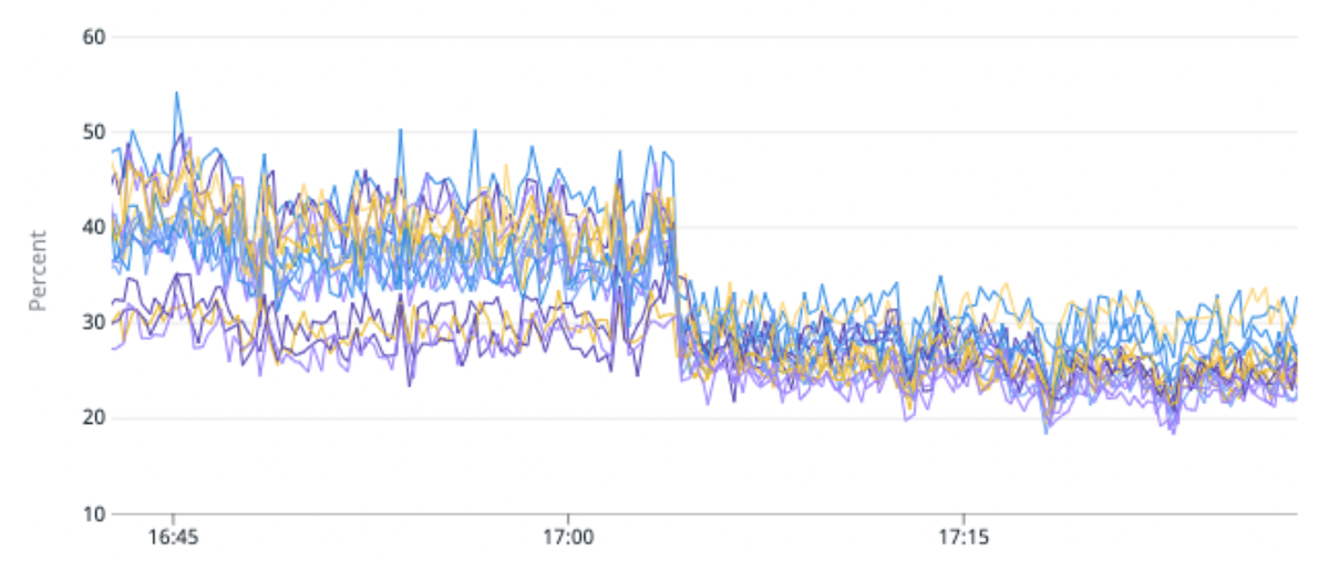
(Fig. 5) 50% improvement in load imbalance and 25% improvement in CPU utilization by migrating a high traffic index to partitions with fewer primary shards per partition.

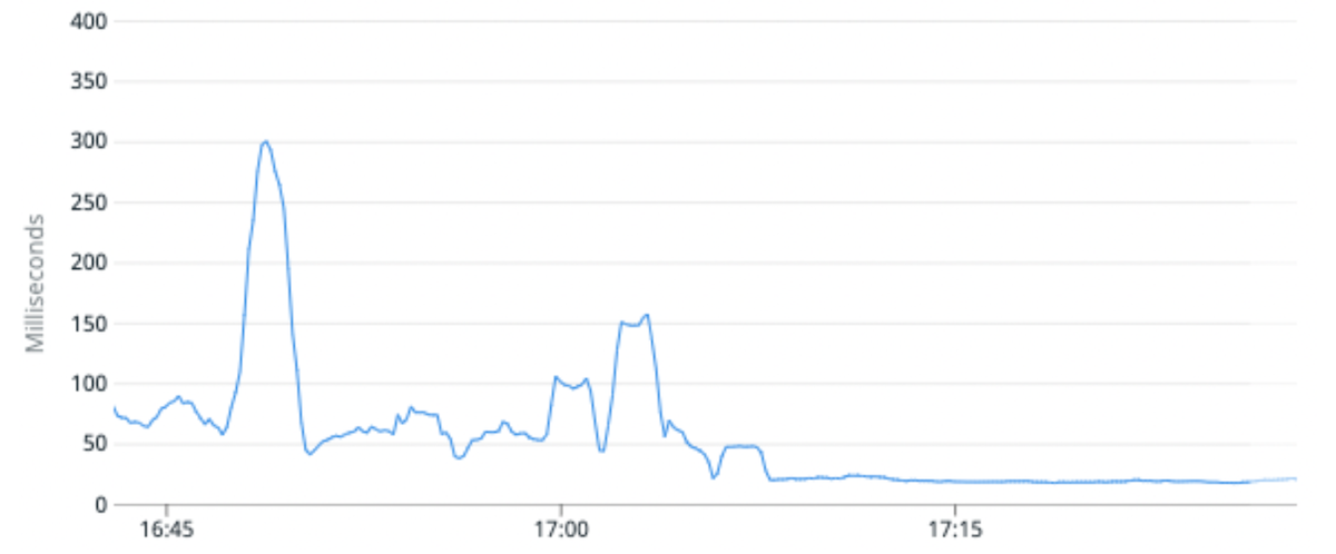
(Fig. 6) Median Request latency improved by 100% on average by migrating a high traffic index to partitions with fewer primary shards per partition.

What’s next?

Introducing Elasticsearch to power new products and features should be straightforward. Our vision is to make it as simple for our engineers to interact with Elasticsearch as modern web frameworks make it to interact with relational databases. It should be easy for teams to create an index, read or write from the index, make changes to its schema, and more – without having to worry about how the requests are served.

Are you interested in the way our Engineering team works at Intercom? Learn more and check out our open roles here.